With the rapid advancement of tracking technologies, the applications of tracking systems in ultrasound imaging he expanded across a wide range of fields. In this review article, we discuss the basic tracking principles, system components, performance analyses, as well as the main sources of error for popular tracking technologies that are utilized in ultrasound imaging. In light of the growing demand for object tracking, this article explores both the potential and challenges associated with different tracking technologies applied to various ultrasound imaging applications, including freehand 3D ultrasound imaging, ultrasound image fusion, ultrasound-guided intervention and treatment. Recent development in tracking technology has led to increased accuracy and intuitiveness of ultrasound imaging and nigation with less reliance on operator skills, thereby benefiting the medical diagnosis and treatment. Although commercially ailable tracking systems are capable of achieving sub-millimeter resolution for positional tracking and sub-degree resolution for orientational tracking, such systems are subject to a number of disadvantages, including high costs and time-consuming calibration procedures. While some emerging tracking technologies are still in the research stage, their potentials he been demonstrated in terms of the compactness, light weight, and easy integration with existing standard or portable ultrasound machines.
Keywords: tracking, ultrasound imaging, optical tracking, electromagnetic tracking, 3D ultrasound imaging, ultrasound–guided interventions, ultrasound image fusion
1. IntroductionAn object tracking system locates a moving object (or multiple objects) through time and space [1]. The main aim of a tracking system is to identify an object regarding the position and orientation in space recorded in an extension of time, characterized by precision, accuracy, working range as well as degree-of-freedom (DOF), depending on the systems and applications [2]. With the rapid development of computational and sensing technologies, nowadays tracking systems he been widely utilized in various fields, including robotics [3,4], military [5,6], medicine [7,8] and sports [9,10]. In the medical field, tracking of rotation and translation of medical instruments or patients plays a substantial role in many important applications, such as diagnostic imaging [11], image-guided nigation systems for intervention and therapy [12,13], as well as rehabilitation medicine [14].
Ultrasound (US) imaging is a well-established imaging modality that has been widely utilized in clinical practice for diagnosing diseases or guiding decision-making in therapy [15]. Compared with other medical imaging modalities, such as computed tomography (CT) and magnetic resonance imaging (MRI), US shows the major advantages of real-time imaging, non-radiation exposure, low-cost, and ease to apply [16]. Despite its many advantages, ultrasonography is considered to be highly operator-dependent [17]. Manually guiding of the US probe to obtain reproducible image acquisition is challenging. Moreover, in order to correctly interpret the information acquired by the scanning, rich clinical experience is required for sonographers. Besides the operator dependency that brings the high risk of interpretive error influencing the diagnosis and therapy results, the restricted field of view (FOV) of US probe poses challenges for image visualization and feature localization, thus limiting diagnosis or therapy accuracy. The integration of object tracking system with US imaging can resolve the above-mentioned limitations. By integrating tracking devices with US probes, an extended FOV of US probe can be obtained, resulting in a less operator-dependent scanning procedure and more accurate results. Over the past decade, there has been a significant growth of studies on integration of various tracking systems with US imaging systems for biomedical and healthcare applications. The applying of emerging tracking systems for biomedical US imaging applications has resulted in improved accuracy and intuitiveness of US imaging and nigation with less reliance on operator skills, thereby benefiting the medical diagnosis and therapy.
The purpose of this article is to provide a literature review on the various tracking systems for biomedical US imaging applications, as illustrated in Figure 1. The rest of the article is organized as follows: in Section 2, the principles of different tracking techniques, including optical tracking, electromagnetic tracking, mechanical tracking, acoustic tracking and inertial tracking, are summarized. The typical tracking systems and their technical performances, such as accuracy and latency are provided in Section 3. Section 4 details the advancement of different tracking systems for US imaging applications, including freehand 3D US imaging, US image fusion, US-guided diagnosis, and US-guided therapy. Finally, a summary and concluding remarks are presented in Section 5.
Figure 1.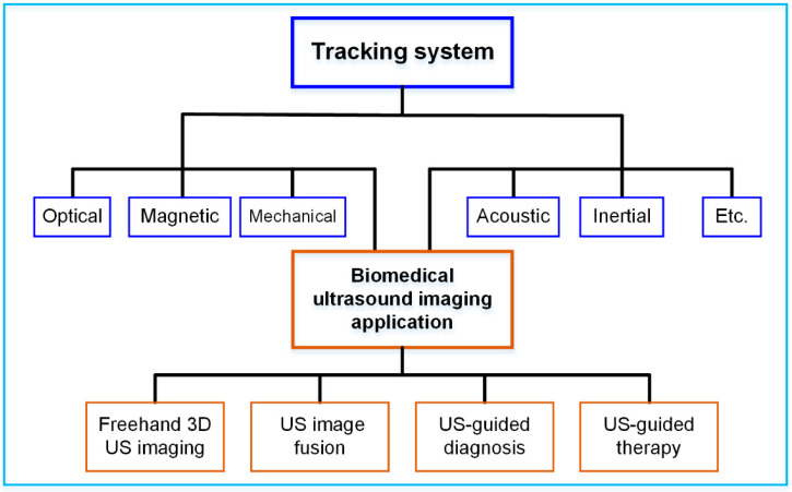
Various tracking systems for biomedical US imaging applications.
2. Physical Principles of Tracking TechnologiesThe latest advancements in tracking technologies he enabled conventional medical devices to be equipped with more advanced functions. In biomedical US imaging, object tracking technologies are key to locate US probes and other medical tools for precise operation and intuitive visualization. The underlying physical principles behind the most common tracking technologies will be reviewed in this section.
2.1. Optical TrackingAn optical tracking system is among the most precise tracking technologies with 6 DOF that achieves a sub-millimeter accuracy level. Multiple spatially synchronized cameras track the markers attached to the target in the designed space. There are two types of markers: active and passive [18]. Infrared light emitting diodes (LEDs) are used in active markers for the purpose of emitting invisible light that can be detected by cameras. A passive marker is covered with a retro-reflective surface that can reflect incoming infrared light back to the camera. There are usually three or more unsymmetrical markers in a target object. The 6 DOF position and orientation of the object are determined by triangulation [19].
Similar to the human vision system, optical tracking requires at least two cameras that are fixed at a known distance from each other. Adding additional cameras will improve tracking accuracy and robustness. In Figure 2, a trinocular vision system is illustrated as an example of triangulation [20]. P is observed simultaneously by three lenses. Additionally, it generates three projection points on the focal plane. A right-handed, Y-up coordinate is assigned to each lens, with coordinate origins at O1, O2, and O3. The reference coordinate XcYcZc coincides with the coordinate X2Y2Z2 of the middle lens. A baseline lij is defined to be the distance between any two lenses. Three parallel principal axes are present in the three fixed lenses. There is a perpendicular relationship between the principal axes and the baseline.
Figure 2.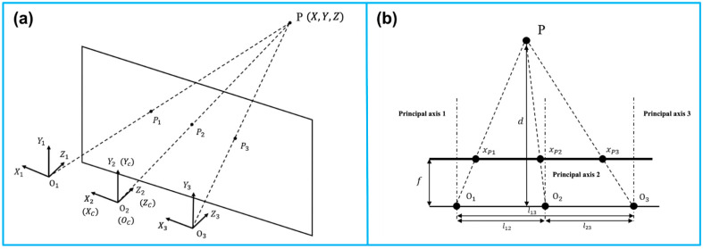
Principle of the camera-based optical tracking technique. (a) The three coordinates represent the three lenses integrated in the camera bar. The camera bar is looking at point P(x, y, z), where P1, P2, and P3 are the intersections on the image plane. (b) The top view demonstrates the similar triangles used to calculate the position information. The depth d of point P can be determined via triangulation. Reprinted from [20] with permission.
To perceive the depth with two lenses i and j, where i, j∈ {1, 2, 3}, and i ≠ j. With the known focal length f, and the disparity xpi−xpj representing the offset between the two projections in the XOZ plane, the depth Z can be derived as
Z=flijxpi−xpj (1)Furthermore, the other two coordinates of P(X,Y,Z) can thus be calculated as
X=xpiZfY=ypjZf (2)Given all the markers’ positions, the orientation of the marker set is determined. With the known positions of all markers, the orientation of the target is also determined. The 6 DOF poser information is delivered in the form of a transformation matrix TMC, with the subscript and superscript representing the marker set coordinate (M) to the camera coordinate (C), respectively.
TMC=[Rp01] (3)where p=(XM,YM,ZM)T is the offset between the two origins of coordinates M and C. Additionally, R is a 3×3 rotational matrix in the form of
R=[cosφcosθcosφsinθsinψ−sinφcosψcosφsinθcosψ+sinφsinψsinφcosθsinφsinθsinψ+cosφcosψsinφsinθcosψ−cosφsinψ−sinθcosθsinψcosθcosψ] (4)From the above matrix, the orientations φ (yaw), θ (pitch), and ψ (roll) can thus be solved as follows:
{φ=arctanR12R11θ=−arcsinR31ψ=arctanR32R33 (5) 2.2. Electromagnetic TrackingTracking systems using electromagnetic signals can also provide sub-millimeter accuracy in dynamic and real-time 6 DOF tracking. Its advantages include being lightweight and free of line-of-sight. In biomedical engineering, it is commonly used for the nigation of medical tools.
Electromagnetic tracking systems consist of four modules: transmission circuits, receiving circuits, digital signal processing units, and microcontrollers. Based on Faraday’s law, electromagnetic tracking systems use transmitted voltages to estimate the position and orientation of objects in alternating magnetic fields when the object is coupled to a receiver sensor [21,22].
Figure 3 illustrates the involved coordinate systems. The reference coordinate system is denoted as X0Y0Z0, which is fixed at the emission coil. XsYsZs is the coordinate system fixed at the receiver sensor. The location of its origin O1(X,Y,Z) with respect to X0Y0Z0, can also be denoted as O1(R,α,β) in spherical coordinate. Additionally, the orientation is represented as Euler angles φ, θ, and ψ.
Figure 3.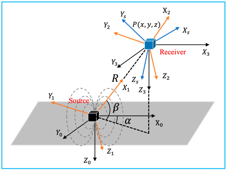
Coordinate systems involved in the 3D electromagnetic tracking (adapted from [21]).
Assuming the excitation current i(t)=Iisin(ωt+ϕ), the transmitter parameter along each direction defined as Ci=μNiIiSi4π, where i=x, y, z, Ni is the number of turns in the coil, and Si is the area of the coil, the excitation signal can be defined as
f0=C=[Cx000Cy000Cz] (6)Accordingly, the receiver parameter can be written as
K=[Kx000Ky000Kz] (7)where ki=ωnigisi, with ω representing the radian frequency of the source excitation signal, ni and si denoting the number of turns in the coil and the area of the coil, and gi indicating the system gain. According to Faraday’s law of induction, the amplitude of the voltage from the receiver coil is expressed as
Sij=ωKjCih(R,α,β,φ,θ,ψ)=ωKjBij (8)With the position and orientation of the receiver fixed, the value of h(R,α,β,φ,θ,ψ) is determined. Bij is the amplitude of the magnetic field produced at that location.
From Equation (8), by defining the final sensor output to be
fs=[sxxsyxszxsxysyyszysxzsyzszz] (9)the magnetic field expressed in XsYsZs is
B=K−1fs=[sxxkxsxykysxzkxsyxkysyykysyzkyszxkzszykzszzkz] (10)When the equivalent transmitter coil along each direction is excited, the square amplitude of the magnetic field P can be expressed as
P=[sxxkx2+syxkx2+szxkx2sxyky2+syyky2+szyky2sxzkz2+syzkz2+szzkz2]=[4Cx2r6(x2+14y2+14z2)4Cy2r6(14x2+y2+14z2)4Cz2r6(14x2+14y2+z2)] (11)Canceling out the unknown position (x, y, z) by summing up all three entries, the only unknown parameter r can be deduced.
With two rotational matrices T(α) and T(β) as
T(α)=[cosαsinα0−sinαcosα0001]T(β)=[cosβ0−sinβ010sinβ0cosβ] (12)A key matrix F can be defined as
F=r6(f0T)−1fsTK−1K−1fsf0−1 =[1+3cos2αcos2β3sinαcosαcos2β−3cosαsinβcosβ3sinαcosαcos2β1+3sin2αcos2α−3sinαsinβcosβ−3cosαsinβcosβ−3sinαsinβcosβ1+3sin2β] (13)As sij, ω, Ci, Kj as known parameters, the unknown α and β can be solved as
{α=arctanF23F13 β=arcsinF33−13 (14)From the spherical coordinates, the position of the target P can be written as
{x=rcosβcosαy=rcosβsinαz=rsinβ (15)Substituting
T(φ)=[1000cosφsinφ0−sinφcosφ]T(θ)=[cosθ0−sinθ010sinθ0cosθ]T(ψ)=[cosψsinψ0−sinψcosψ0001] (16)into
fs=KB=2r3KT(φ)T(θ)T(ψ)T(−α)T(−β)ST(β)T(α)f0 (17)matrix T is defined as
T=T(φ)T(θ)T(ψ)=[cosφcosψcosφsinψ−sinφsinθsinφcosψ−cosθsinψsinφsinθsinψ+cosθcosψsinθcosφcosθsinφcosψ+sinθsinψcosθsinφsinψ+sinθcosψcosθcosφ] (18)Therefore, the target’s orientation can be solved as
{φ=arctan(−T13(T232+T332)12)θ=arctan(T23T33) ψ=arctan(T12T11) (19) 2.3. Mechanical TrackingRobotic tracking systems use articulated robotic arms to manipulate the target attached to the end effector. Typically, industrial robots are composed of a number of joints and links. Joint movement is continuously detected by potentiometers and encoders in-stalled on each joint. The real-time position and orientation of the effector can be deter-mined by calculating homogeneous transformations from the collected robotic dynamics. In clinical practice, the operator can either control the movement of the robot to a certain location with the desired orientation, or specify the destination, and the robot solves the path using inverse dynamics based on the spatial information of the destination and the architecture of the robot. Following the Denit and Hartenberg notation, the forward dynamics will be applied to illustrate how the 6 DOF pose information is transformed be-tween adjacent joints and links, as illustrated in Figure 4 [23].
Figure 4.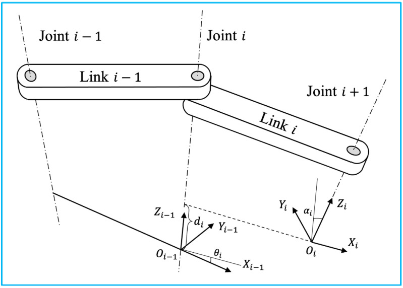
Two adjacent links with a revolute joint with the relative position denoted using Denit-Hartenberg convention (adapted from [23]).
The 4×4 homogeneous transformation matrix for each step is shown below.
A1=[cosθi−sinθi00sinθicosθi0000100001], A2=[100ai010000100001]A3=[10000100001di0001], A1=[10000cosαi−sinαi00sinαicosαi00001] (20) [xiyizi1]=A1A2A3A4⏟T[xiyizi1]=[cosθi−sinθicosαisinθisinαiaicosθisinθicosθicosαi−cosθisinαiaisinθi0sinαicosαidi0001][xiyizi1] (21)The transformation matrix T can also be represented in terms of position (px,py,pz) in the reference coordinate and orientation (φ,θ,ψ) in yaw-pitch-roll representation.
T=[cosφcosθcosφsinθsinψ−sinφcosψcosφsinθcosψ+sinφsinψpxsinφcosθsinφsinθsinψ+cosφcosψsinφsinθcosψ−cosφsinψpy−sinθcosθsinψcosθcosψpz0001] (22)Based on Equations (21) and (22), the 6 DOF pose information can be solved as
{px=aicosθipy=aisinθipz=di (23) {θ=arcsin(−T31)φ=arccos(T33cosθ)ψ=arccos(T11cosθ) (24) 2.4. Acoustic TrackingAn acoustic tracking system is one of the three DOF positional tracking systems. To determine the spatial location of the target object, an ultrasonic transmitter transmits a carrier signal that is received by multiple receivers operating at the same frequency. Specifically, by estimating the actual trel/arrival times (TOF/TOA) or the time difference between trel/arrival (TDOF/TDOA), the 3D coordinates of the object (x, y, z) can be determined to centimeter accuracy levels with receivers fixed at known locations, as shown in Figure 5. A TDOF/TDOA algorithm is more practical and accurate than a TOF/TOA algorithm since it circumvents the synchronization issue between the transmitter and receiver. A limitation of acoustic tracking is that the accuracy of the tracking is affected by the temperature and air turbulence in the environment [24]. This problem can be addressed by including the speed of sound (c) as an unknown parameter in the calculation [25].
Figure 5.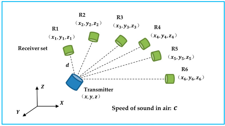
The transmitter sends out carrier signals to the receiver set. The unknow transmitter’s position and the speed of sound can be solved based of the time difference of arrival.
The predetermined geometry of the receivers was notated as (xi,yi,zi), where i represents the ith receiver, where i {1, 2, 3, 4, 5, 6}. The reference distance between the transmitter and receiver R1 is denoted as d. ΔT1j indicates the TDOF between receiver R1 and Rj, where j∈ {2, 3, 4, 5, 6}.
[2x1−2x22y1−2y22z1−2z2−2ΔT12−2ΔT1222x1−2x32y1−2y32z1−2z3−2ΔT13−2ΔT1322x1−2x42y1−2y42z1−2z4−2ΔT14−2ΔT1422x1−2x52y1−2y52z1−2z5−2ΔT15−2ΔT1522x1−2x62y1−2y62z1−2z6−2ΔT16−2ΔT162][xyzcdc2]=[x12+y12+z12−x22−y22−z22x12+y12+z12−x32−y32−z32x12+y12+z12−x42−y42−z42x12+y12+z12−x52−y52−z52x12+y12+z12−x62−y62−z62] (25)Occlusion can also affect the accuracy of an acoustic tracking system. A receiver configuration should be taken into serious consideration when implementing such a system for biomedical US imaging applications [26]. In addition to reducing occlusion, an optimal configuration also contributes to improved tracking performance. As an acoustic tracking system is not able to identify a target’s object, other tracking systems, such as inertial tracking, are frequently required [27].
2.5. Inertial TrackingInertial tracking systems are based on an inertial measurement unit (IMU), which is a small, lightweight, cost-effective sensor enabled by microelectromechanical systems (MEMS) (Figure 6) [28]. An IMU sensor with 9 axes that integrates accelerometers, gyroscopes, and magnetometers is commonly used for 6 DOF object tracking. Accelerometers measure the target’s acceleration. The angular velocity of a target is measured by a gyroscope. Additionally, a magnetometer detects the magnetic field strength at the target’s location. With sensor fusion of the raw measurements, an IMU sensor is able to obtain more accurate readings [29]. As a result, after calibration and compensation for drifts and errors, the position and orientation of the target can be determined [27].
Figure 6.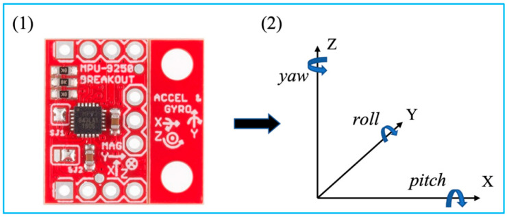
MPU 9250 and its coordinate system with Euler angles. Reprinted from [27] with permission.
The tri-axial measurements of the accelerometer are accelerations of each axis, where a=[ax,ay,az]T=[d2xdt2,d2ydt2,d2zdt2]T. Readings from the gyroscope indicate the angular rates of the sensor when rotated, where ω=[ωx,ωy,ωz]T=[d2φdt2,d2θdt2,d2ψdt2]T. Additionally, [pitch,roll,yaw]T is denoted as Φ=[φ,θ,ψ]T.
By taking integration of the angular velocity from time tk−1 to tk,
Φ=∫tk−1tkmω(τ) d (26)where τ is the discrete time. The solution of the orientation, under the assumption, can be written as
Φ=ωk−1+ωk2(tk−tk−1) (27)For simplicity, three rotation matrices were defined as follows.
Rpitch=[cosθ0−sinθ010sinθ0cosθ] Rroll=[1000cosψsinψ0−sinψcosψ] Ryaw=[cosφ−sinφ0sinφcosφ0001]The rotational matrix R is expressed as
R=Rpitch⋅Rroll⋅Ryaw (28)Due to the effect of the Earth’s grity,
υ˙=Ra−g (29)where υ is the velocity of the object and g=[0,0,9.8]T.
According to the midpoint method, the velocity
υk=υk−1+(Rk−1ak−1+Rkak2−g)(tk−tk−1) (30)Thus, the position p=[x,y,z]T at time k is
pk=pk−1+υk−1(tk−tk−1)+12(Rk−1ak−1+Rkak2−g)(tk−tk−1)2 (31) 3. Tracking SystemsDifferent types of tracking systems he been developed and marketed over the past decade. In this section, the main tracking systems in the market are reviewed in terms of their technical specifications.
3.1. Optical Tracking SystemsA large number of manufacturers he developed various kinds of optical tracking systems for biomedical applications, as summarized in Table 1. The main technical specifications that relate to the tracking performances are measurement volume (or FOV), resolution, volumetric accuracy, erage latency, and measurement rates. Due to angle of view, the shape of measurement volume is usually a pyramid, which can be represented by radius × width × height. Some manufacturers prefer to use the term “field of view”, i.e., horizontal degree × vertical degree, to show the dimension of work volume. In addition, the advances of cameras promote the resolution of the image, and further increase the volumetric accuracy. To date, some advanced optical tracking system can obtain 26 megapixels (MP) resolution with 0.03 mm volumetric accuracy [30]. However, the high resolution of the captured images will burden the processor for data analysis, causing the increase of erage latency and reduce of measurement rates.
Table 1.Summary of commercially ailable optical tracking systems.
Manufacturer Model Measurement Volume (Radius × Width × Height) orFOV Resolution Volumetric Accuracy (RMS) Average Latency Measurement Rate Northern Digital Inc., Waterloo, ON, Canada Polaris Vega ST [31] 2400 × 1566 × 1312 mm3 (Pyramid Volume:)3000 × 1856 × 1470 mm3 (Extended Pyramid) N/A 0.12 mm (Pyramid Volume)0.15 mm (Extended Pyramid)