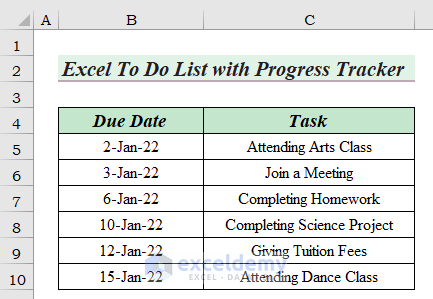
The following table contains the Due Date and Task columns. We will use it to create a progress tracker.
Method 1 – Using “To-Do List with Progress Tracker” Template
Steps:
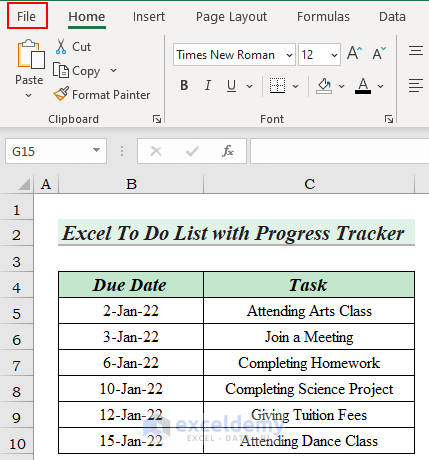
Go to the File tab.
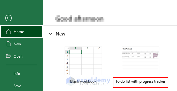
Select the To Do list with progress tracker template.
If you can’t find the option, go to “More templates” and search for “progress tracker”.
Click on Create.
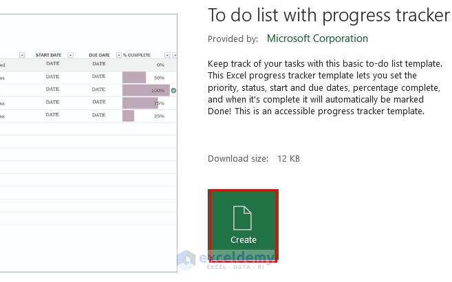
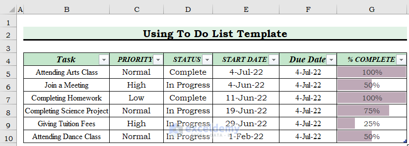
The template loads in our Excel sheet.
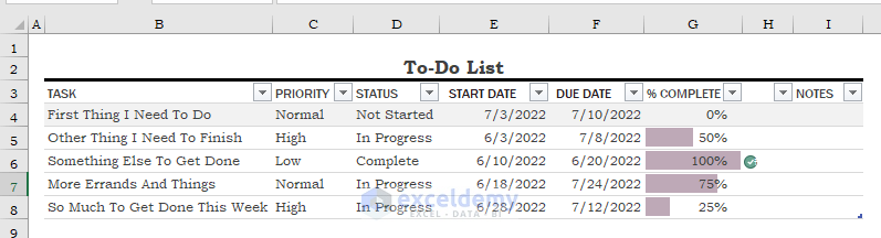
Manually input the information from the dataset.
Method 2 – Use of Conditional Formatting Feature to Create a To-Do List with Progress Tracker
We will insert a check box in the Status column and use it for the formatting.
Inserting Check Box
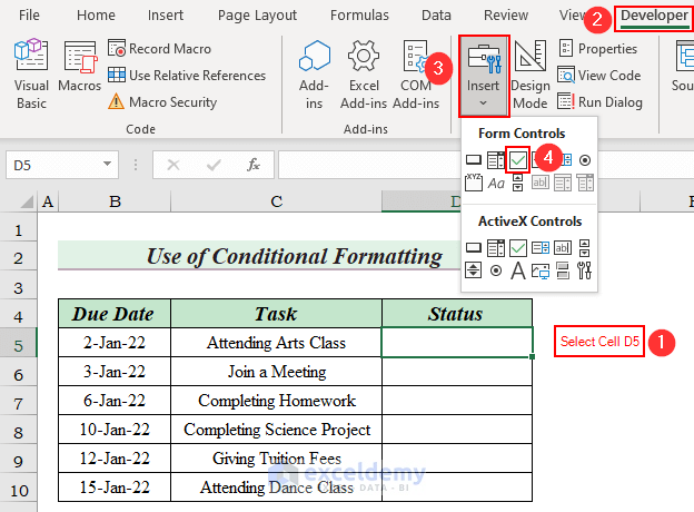
Select cell D5.
Go to the Developer tab and select Insert.
From Form Controls, select the check box icon.
Drag down the check box with the Fill Handle tool to complete the column.

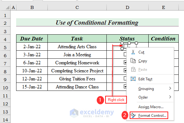
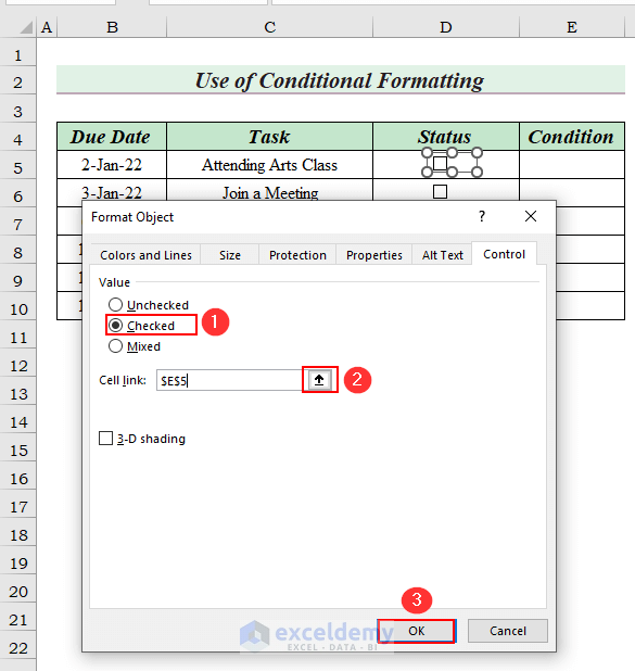
Right-click on the check box of cell D5.
Select Format Control from the Context Menu. A Format Object dialog box will appear.
Select Checked as Value and cell E5 as Cell Link
Click OK.
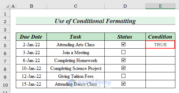
You can see the Condition of cell D5 is TRUE, as the cell box is marked.
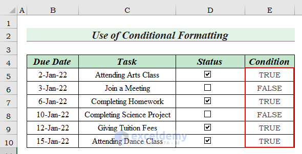
Repeat for other cells to complete the Condition column.
You can see Condition is FALSE when the check box is unmarked.
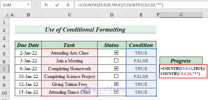
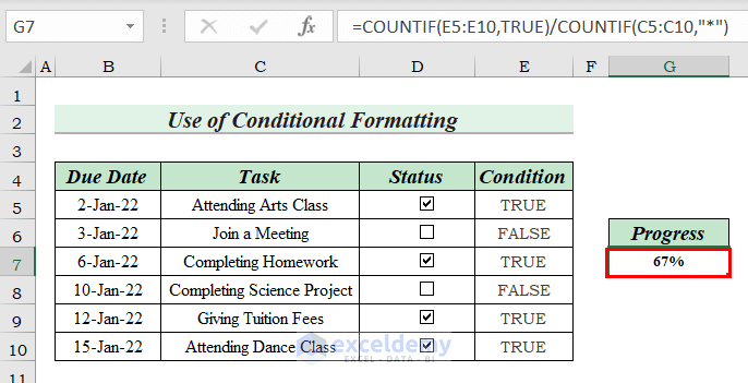
Now, we will calculate Progress.
Type the following formula in cell G7.
=COUNTIF(E5:E10,TRUE)/COUNTIF(C5:C10,"*")
Formula Breakdown
COUNTIF(E5:E10,TRUE) → The COUNTIF function counts the number of cells that he TRUE.
Output: 4
COUNTIF(C5:C10,”*”) → counts the number of cells that he a criterion.
Output: 6
COUNTIF(E5:E10,TRUE)/COUNTIF(C5:C10,”*”) is dividing 4 by 6.
Output: 67%.
Press Enter.
Inserting Progress Tracker
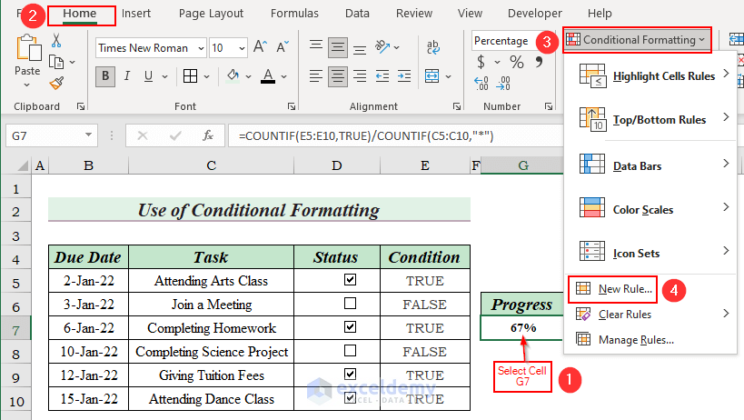
Select cell G7 and go to the Home tab.
In Conditional Formatting, select New Rule. A New Formatting Rule dialog box will appear.
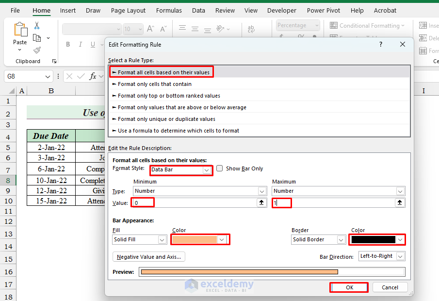
Select Format all cells based on their values.
Click on the drop-down arrow of the Format Style box and select Data Bar.
Click on the drop-down arrow of the Minimum and select Number and set the Value as 0.
Click on the drop-down arrow of the Maximum and select Number, and set the Value as 1.
Click on the drop-down arrow of the Border box and select Solid Border.
Select Bar Direction as Left to Right and select a Color.
Click on OK.
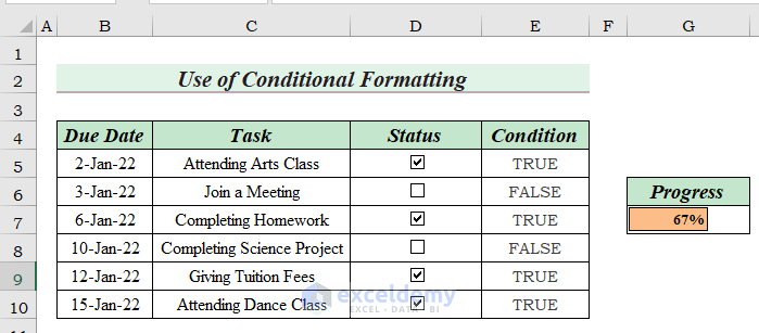
As a result, we can see the Excel to do list with progress tracker.
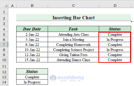
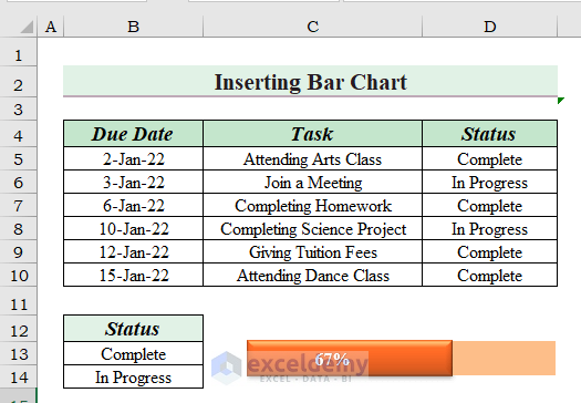
Method 3 – Inserting Bar Chart to Create Progress Tracker
We will customize the Status column with Data validation and use it for the bar chart.
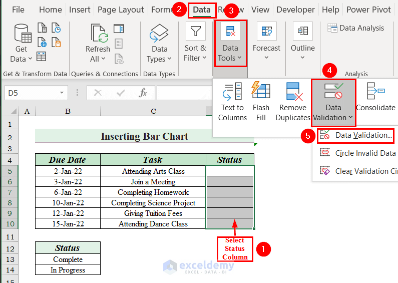
Completing Status Column
Put status text in the cells B13 and B14.
Select the Status column cells.
Go to the Data tab and select Data Tools.
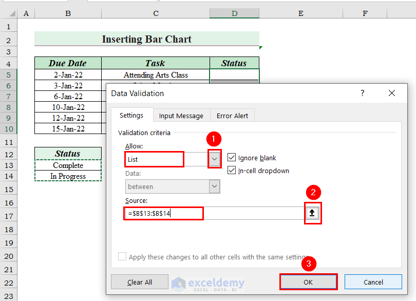
From Data Validation, select Data Validation. A Data Validation dialog box will appear.
Click on the drop-down arrow of the Allow box and select List.
Click on the upward arrow of the Source box and select cells B13 and B14 as Source.
Press OK.
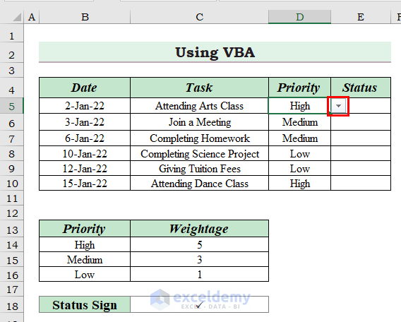
When we click on cell D5, we can see a drop down arrow on the top right side of cell D5.
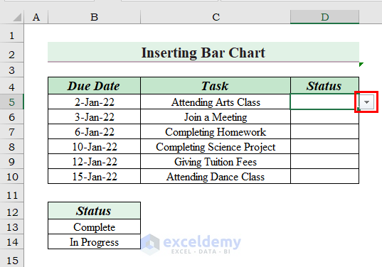
Click on the drop-down arrow of cell D5 and can select a status.
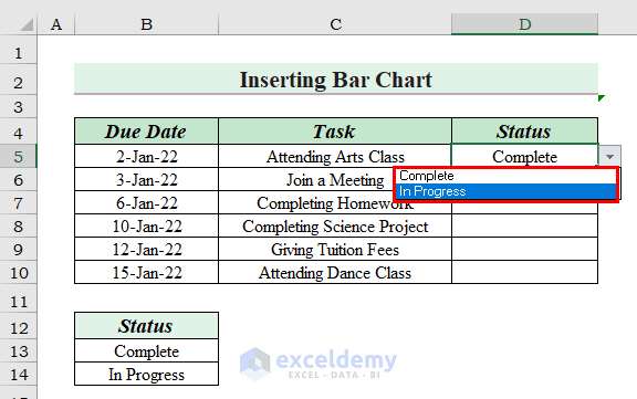
Fill in the Status column.
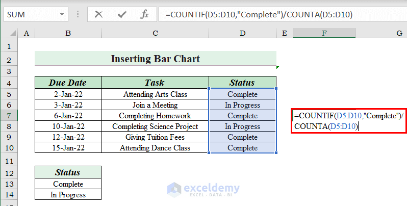
Progress Calculation
Use the following formula in cell F7:
=COUNTIF(D5:D10,"Complete")/COUNTA(D5:D10)
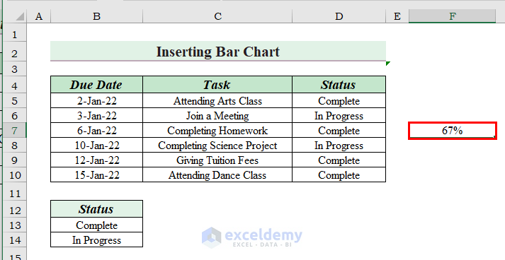
Formula Breakdown
COUNTIF(D5:D10,”Complete”) → counts the number of cells that he COMPLETE.
Output: 4
COUNTA(D5:D10) → the COUNTA function counts the number of cells between D5 and D10.
Output: 6
COUNTIF(D5:D10,”Complete”)/COUNTA(D5:D10) is dividing 4 by 6.
Output: 67%.
Press Enter.
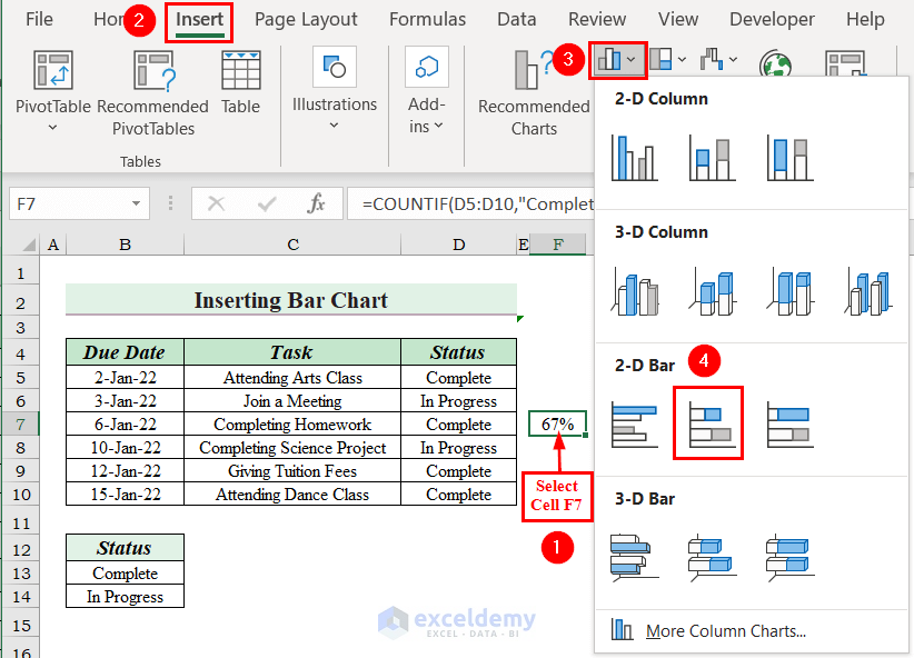
Inserting Bar Chart
Click on cell F7 and go to the Insert tab.
From Bar chart, select Stacked Bar chart.
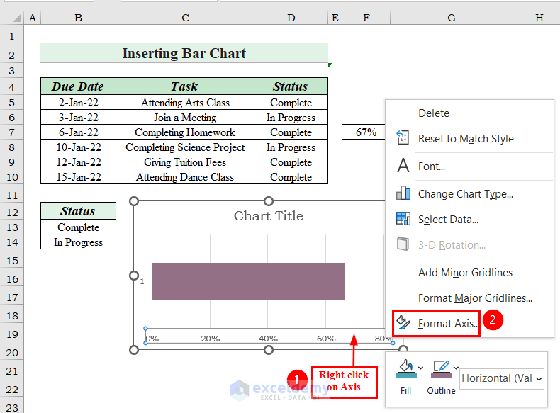
Right-click on the chart Axis.
From the Context Menu, select Format Axis. A Format Axis dialog box will appear on the right side of the Excel sheet.
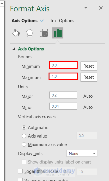
In the Bounds option, put Minimum as 0 and Maximum as 1.
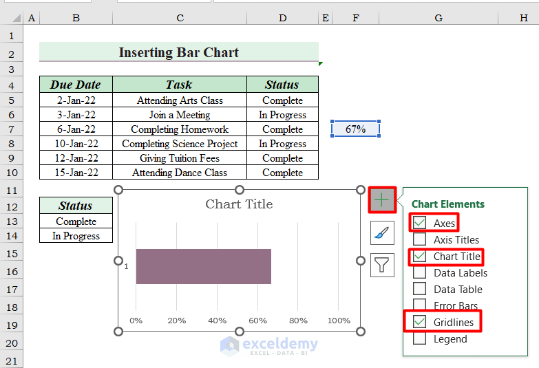
Click on the Chart Elements and unmark Axes, Chat Title, and Gridlines.
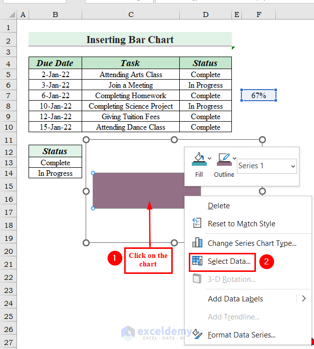
Click on the Chart and choose Select Data from the Context Menu. A Select Data Source dialog box will appear.
Click on Add. An Edit Series dialog box will appear.
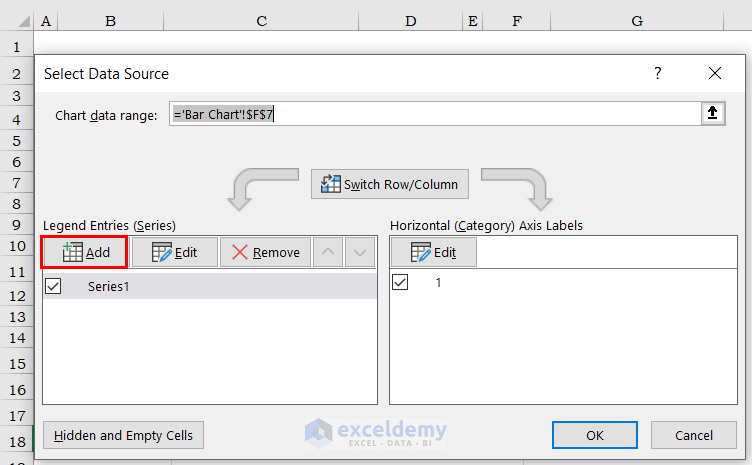
Set the Series value as 1 and click OK.
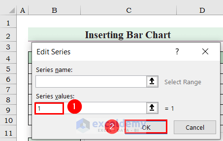
Make sure Series1 is above Series2.
Click OK.
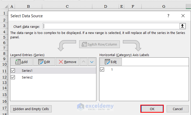
You can see two shades of the Bar chart has been created and overlapped on one another.
Click on the first half of the Bar chart.
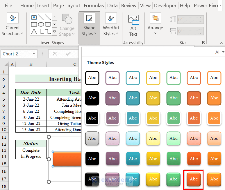
Go to the Format tab and select Shape Styles.
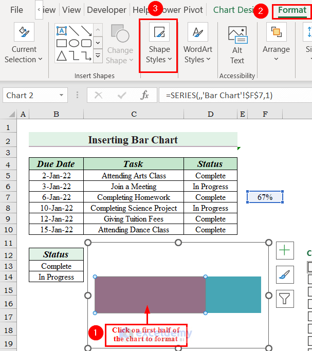
Hover over Themes and see the preview on the Bar chart. Then select a Theme you want to use. We selected Orange colored Theme.
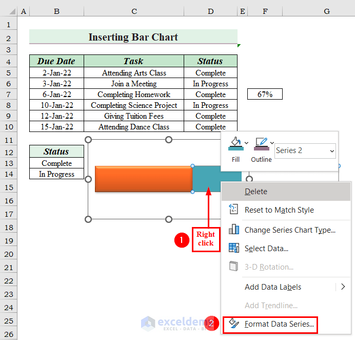
Right-click on the other portion of the Bar chart and select Format Data Series.
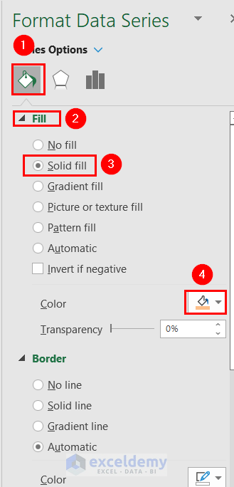
From the Format Data Series dialog box, select Fill.
Select Solid Fill and choose a Color. Here, we selected a lighter orange shade.
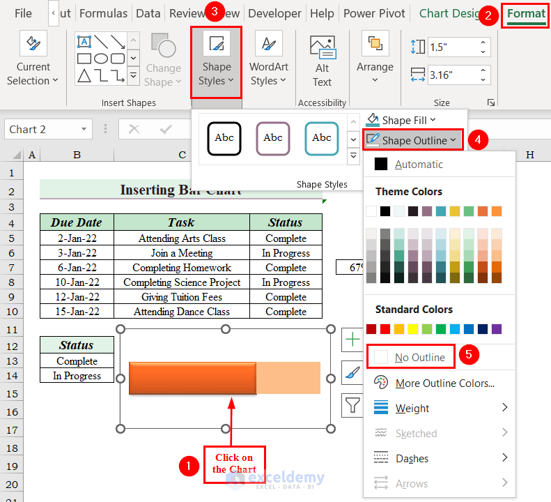
Click on the Bar chart and go to the Format tab.
Select Shape Styles.
From Shape Outline, select No Outline.
Adding Progress:
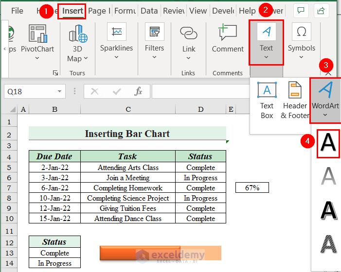
Go to the Insert tab and select the Text option.
From WordArt, select the first option.
Click on the Text box and go to the Formula Bar.
Type “=” and select cell F7.
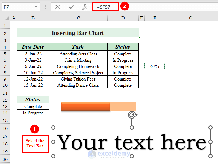
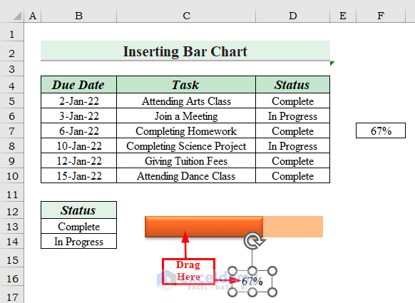
Drag this Text box to the Bar chart.
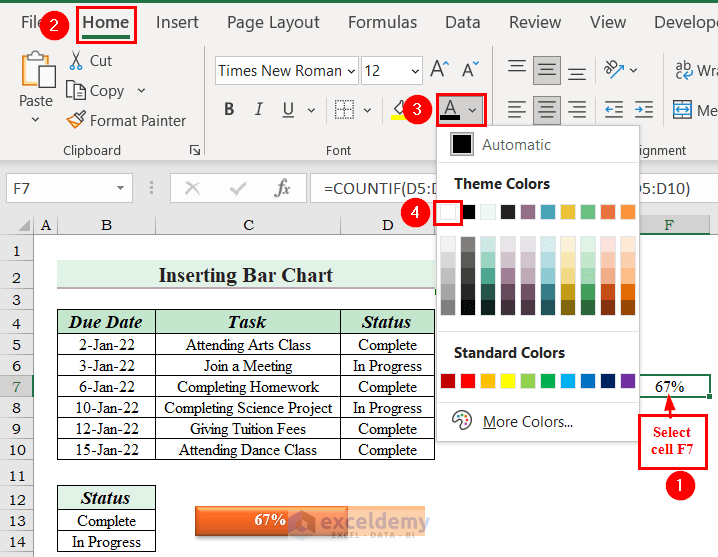
Make the text bold and change the color font to white.
Click on cell F7.
Go to the Home tab and Font Color, then select White.
As a result, we can see a complete Excel to do list with progress tracker.
Method 4 – Using VBA to Create To-Do List with Progress Tracker in Excel
Let’s create a Priority list and insert a Status Input symbol tables to use as reference (see picture below).
Steps:
Create the Priority column by following Method 3.
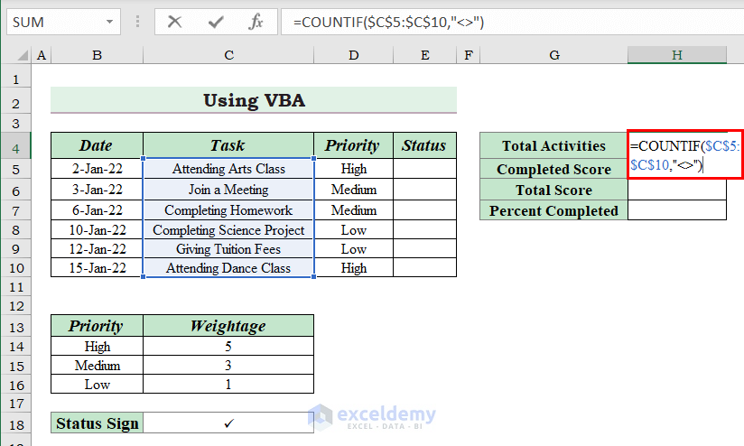
Type the following formula in cell H4 to calculate Total Activities and press Enter:
=COUNTIF($C$5:$C$10,"")
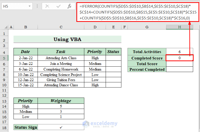
Type the following formula in cell H5 to calculate the Completed Score and press Enter:
=IFERROR(COUNTIFS($D$5:$D$10,$B$14,$E$5:$E$10,$C$18)*$C$14+COUNTIFS($D$5:$D$10,$B$15,$E$5:$E$10,$C$18)*$C$15+COUNTIFS($D$5:$D$10,$B$16,$E$5:$E$10,$C$18)*$C$16,0)
Formula Breakdown
COUNTIFS($D$5:$D$10,$B$14,$E$5:$E$10,$C$18) → the COUNTIFS function applies the criterion to cells across multiple ranges and counts the number of times the criterion is met.
Output: 0
COUNTIFS($D$5:$D$10,$B$14,$E$5:$E$10,$C$18)*$C$14 → multiplies 0 with $C$14.
Output: 0
COUNTIFS($D$5:$D$10,$B$15,$E$5:$E$10,$C$18) → applies criterion to cells across multiple ranges and counts the number of times the criterion is met.
Output: 0
COUNTIFS($D$5:$D$10,$B$15,$E$5:$E$10,$C$18)*$C$15→ multiplies 0 with $C$15.
Output: 0
COUNTIFS($D$5:$D$10,$B$16,$E$5:$E$10,$C$18) → applies criterion to cells across multiple ranges and counts the number of times the criterion is met.
Output: 0
COUNTIFS($D$5:$D$10,$B$16,$E$5:$E$10,$C$18)*$C$16 → multiplies 0 with $C$16.
Output: 0
IFERROR(COUNTIFS($D$5:$D$10,$B$14,$E$5:$E$10,$C$18)*$C$14+COUNTIFS($D$5:$D$10,$B$15,$E$5:$E$10,$C$18)*$C$15+COUNTIFS($D$5:$D$10,$B$16,$E$5:$E$10,$C$18)*$C$16,0) → the IFERROR function returns the value of the formula, otherwise returns 0 when there is an error in the formula.
Output: 0
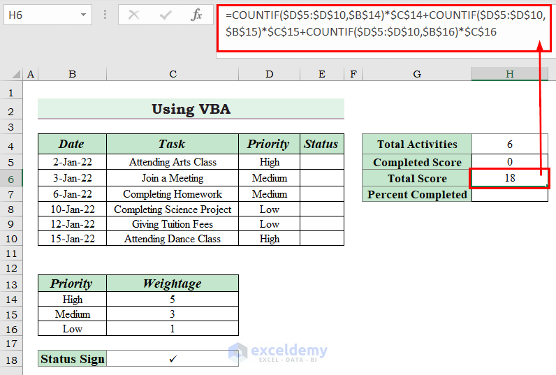
Use the following formula in cell H6 and press Enter.
=COUNTIF($D$5:$D$10,$B$14)*$C$14+COUNTIF($D$5:$D$10,$B$15)*$C$15+COUNTIF($D$5:$D$10,$B$16)*$C$16
Formula Breakdown
COUNTIF($D$5:$D$10,$B$14) → counts the number of cells that meets a criterion
Output → 2
COUNTIF($D$5:$D$10,$B$14)*$C$14 → multiplies 2 with $C$14
Output → 10
COUNTIF($D$5:$D$10,$B$15) → counts the number of cells that meet a criterion
Output → 2
COUNTIF($D$5:$D$10,$B$15)*$C$15 → multiplies 2 with $C$15
Output → 6
COUNTIF($D$5:$D$10,$B$16) → counts the number of cells that meet a criterion
Output → 2
COUNTIF($D$5:$D$10,$B$16)*$C$16 → multiplies 2 with $C$16
Output → 2
COUNTIF($D$5:$D$10,$B$14)*$C$14+COUNTIF($D$5:$D$10,$B$15)*$C$15+COUNTIF($D$5:$D$10,$B$16)*$C$16 →Therefore, it becomes
Output → 18
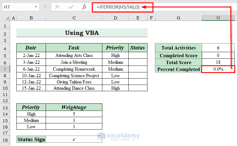
Use the following formula in cell H7 and apply it with Enter.
=IFERROR(H5/H6,0)
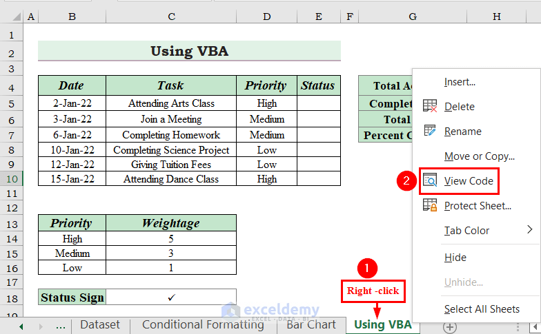
Right-click on the sheet name.
Select View Code from the Context Menu. A VBA editor window will appear.
Select Worksheet.
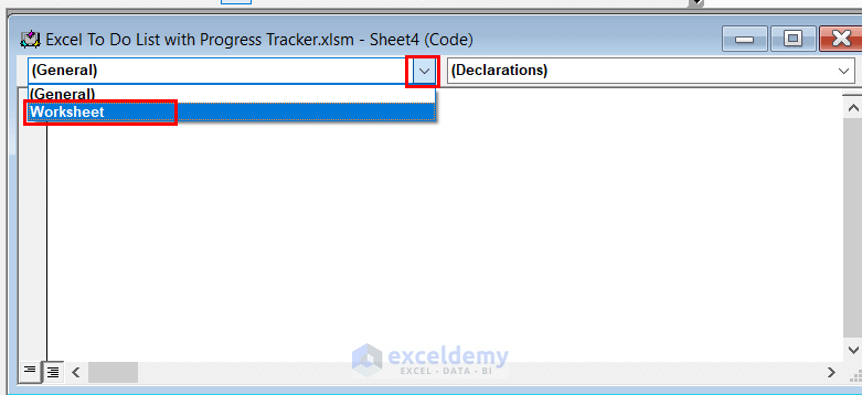
Select BeforeDoubleClick under SelectionChange.
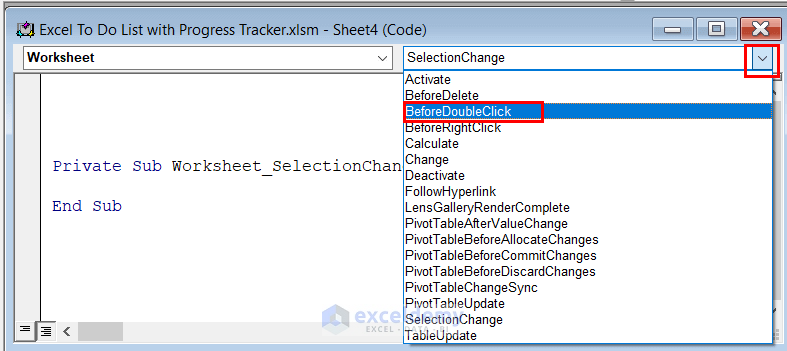
Copy the following code in the VBA editor window.
Private Sub Worksheet_BeforeDoubleClick(ByVal Target As Range, Cancel As Boolean)
Cancel = False
If Target.Row >= 5 And Target.Row