Perceiving, maintaining, and using time intervals in working memory are crucial for animals to anticipate or act correctly at the right time in the ever-changing world. Here, we systematically study the underlying neural mechanisms by training recurrent neural networks to perform temporal tasks or complex tasks in combination with spatial information processing and decision making. We found that neural networks perceive time through state evolution along stereotypical trajectories and produce time intervals by scaling evolution speed. Temporal and nontemporal information is jointly coded in a way that facilitates decoding generalizability. We also provided potential sources for the temporal signals observed in nontiming tasks. Our study revealed the computational principles of a number of experimental phenomena and provided several predictions.
Keywords: interval timing, population coding, neural network model
AbstractTo maximize future rewards in this ever-changing world, animals must be able to discover the temporal structure of stimuli and then anticipate or act correctly at the right time. How do animals perceive, maintain, and use time intervals ranging from hundreds of milliseconds to multiseconds in working memory? How is temporal information processed concurrently with spatial information and decision making? Why are there strong neuronal temporal signals in tasks in which temporal information is not required? A systematic understanding of the underlying neural mechanisms is still lacking. Here, we addressed these problems using supervised training of recurrent neural network models. We revealed that neural networks perceive elapsed time through state evolution along stereotypical trajectory, maintain time intervals in working memory in the monotonic increase or decrease of the firing rates of interval-tuned neurons, and compare or produce time intervals by scaling state evolution speed. Temporal and nontemporal information is coded in subspaces orthogonal with each other, and the state trajectories with time at different nontemporal information are quasiparallel and isomorphic. Such coding geometry facilitates the decoding generalizability of temporal and nontemporal information across each other. The network structure exhibits multiple feedforward sequences that mutually excite or inhibit depending on whether their preferences of nontemporal information are similar or not. We identified four factors that facilitate strong temporal signals in nontiming tasks, including the anticipation of coming events. Our work discloses fundamental computational principles of temporal processing, and it is supported by and gives predictions to a number of experimental phenomena.
Much information that the brain processes and stores is temporal in nature. Therefore, understanding the processing of time in the brain is of fundamental importance in neuroscience (1–4). To predict and maximize future rewards in this ever-changing world, animals must be able to discover the temporal structure of stimuli and then flexibly anticipate or act correctly at the right time. To this end, animals must be able to perceive, maintain, and then use time intervals in working memory, appropriately combining the processing of time with spatial information and decision making (DM). Based on behioral data and the diversity of neuronal response profiles, it has been proposed (5, 6) that time intervals in the range of hundreds of milliseconds to multiseconds can be decoded through neuronal population states evolving along transient trajectories. The neural mechanisms may be accumulating firing (7, 8), synfire chains (9, 10), the beating of a range of oscillation frequencies (11), etc. However, these mechanisms are challenged by recent finding that animals can flexibly adjust the evolution speed of population activity along an invariant trajectory to produce different intervals (12). Through behioral experiments, it was found that humans can store time intervals as distinct items in working memory in a resource allocation strategy (13), but an electrophysiological study on the neuronal coding of time intervals maintained in working memory is still lacking. Moreover, increasing evidence indicates that timing does not rely on dedicated circuits in the brain but instead, is an intrinsic computation that emerges from the inherent dynamics of neural circuits (3, 14). Spatial working memory and DM are believed to rely mostly on a prefrontoparietal circuit (15, 16). The dynamics and the network structure that enable this circuit to combine spatial working memory and DM with flexible timing remain unclear. Overall, our understanding of the processing of time intervals in the brain is fragmentary and incomplete. It is, therefore, essential to develop a systematic understanding of the fundamental principle of temporal processing and its combination with spatial information processing and DM.
The formation of temporal signals in the brain is another unexplored question. Strong temporal signals were found in the brain even when monkeys performed working memory tasks where temporal information was not needed (17–21). In a vibrotactile working memory task (17), monkeys were trained to report which of the two vibrotactile stimuli separated by a fixed delay period had higher frequency (Fig. 1D). Surprisingly, although the duration of the delay period was not needed to perform this task, temporal information was still coded in the neuronal population state during the delay period, with the time-dependent variance explaining more than 75% of the total variance (18, 19). A similar scenario was also found in other nontiming working memory tasks (19–21). It is unclear why such strong temporal signals arose in nontiming tasks.
Fig. 1.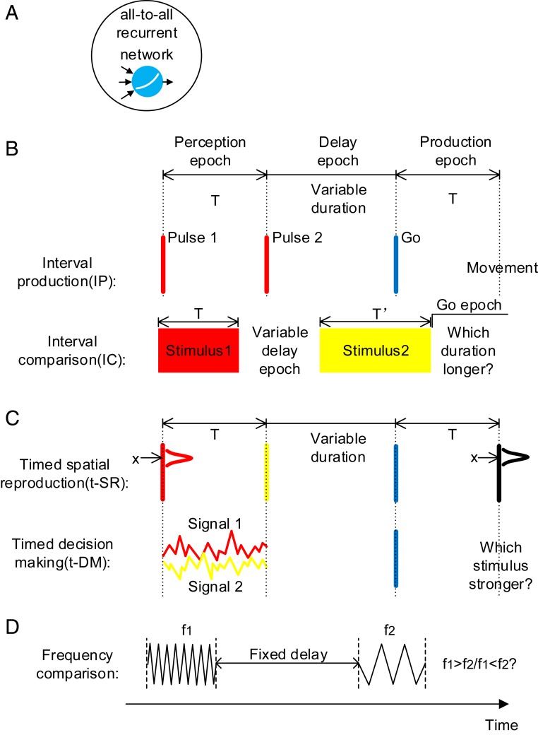
Model setup. (A) All-to-all connected recurrent networks with soft plus units are trained. (B) Basic timing tasks. IP: The duration T of the perception epoch determines the movement time after the go cue. IC: The duration T of the stimulus 1 epoch is compared with the duration T′ of the stimulus 2 epoch. Stimuli with different colors (red, yellow, or blue) indicate that they are input to the network through different synaptic weights. (C) Combined timing tasks. T determines the movement time after the go cue. Spatial location (t-SR) or decision choice (t-DM) determines the movement behior. (D) A nontiming task in the experimental study (18). Although the duration of the delay period is not needed to perform the task, there exists strong temporal signals in the delay period.
Previous works showed that, after being trained to perform tasks such as categorization, working memory, DM, and motion generation, artificial neural networks (ANNs) exhibited coding or dynamic properties surprisingly similar to experimental observations (22–25). Compared with animal experiments, ANN can cheaply and easily implement a series of tasks, greatly facilitating the test of various hypotheses and the capture of common underlying computational principles (26, 27). In this paper, we trained recurrent neural networks (RNNs) (Fig. 1A) to study the processing of temporal information. First, by training networks on basic timing tasks, which require only temporal information to perform (Fig. 1B), we studied how time intervals are perceived, maintained, and used in working memory. Second, by training networks on combined timing tasks, which require both temporal and nontemporal information to perform (Fig. 1C), we studied how the processing of time is combined with spatial information processing and DM, the influence of this combination on decoding generalizability, and the network structure that this combination is based on. Third, by training networks on nontiming tasks (Fig. 1D), we studied why such a large time-dependent variance arises in nontiming tasks, thereby understanding the factors that facilitate the formation of temporal signals in the brain. Our work presents a thorough understanding of the neural computation of time.
ResultsWe trained an RNN of 256 soft plus units supervisedly using back propagation through time (28). Self-connections of the RNN were initialized to one, and off-diagonal connections were initialized as independent Gaussian variables with mean of zero (27), with different training configurations initialized using different random seeds. The strong self-connections supported self-sustained activity after training (SI Appendix, Fig. S1B), and the nonzero initialization of the off-diagonal connections induced sequential activity comparable with experimental observations (27). We stopped training as soon as the performance of the network reached criterion (23, 25) (performance examples are in SI Appendix, Fig. S1).
Basic Timing Tasks: Interval Production and Interval Comparison Tasks. Interval production task.In the interval production (IP) task (the first task of Fig. 1B), the network was to perceive the interval T between the first two pulses, maintain the interval during the delay epoch with variable duration, and then produce an action at time T after the go cue. Neuronal activities after training exhibited strong fluctuations (Fig. 2A). In the following, we report on the dynamics of the network in the perception, delay, and production epochs of IP (Fig. 1 has an illustration of these epochs).
Fig. 2.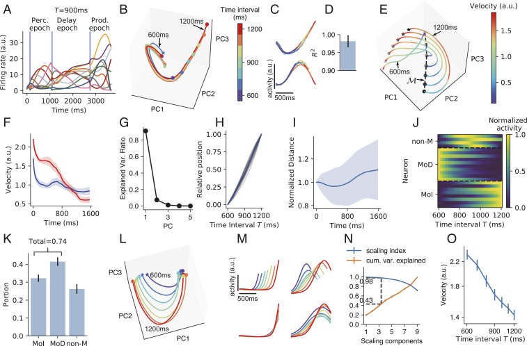
IP task. (A) The activities of example neurons (indicated by lines of different colors) when the time interval T between the first two pulses is 900 ms. Vertical blue shadings indicate the pulse input to the network. (B) Population activity in the perception epoch in the subspace of the first three PCs. Colors indicate the time interval T. Stars and circles indicate the starting and ending points of the perception epoch, respectively. The trajectories for T=600 and 1,200 ms are labeled. (C) Firing profiles of two example neurons in the perception epoch. Line colors he the same meaning as in B. (D) Coefficient of determination (R2) of how much the neuronal firing profile with the largest T can explain the variance of the firing profiles with smaller T in the perception epoch. Error bar indicates SD over different neurons and T values. (E) Population activity in the subspace of the first three PCs in the delay epoch. Colors indicate trajectory speed. The increasing blackness of stars and circles indicates trajectories with T=600, 700⋯ 1,200 ms. The dashed curve connecting the end points of the delay epoch marks manifold M. (F) Trajectory speed as a function of time in the delay epoch when T=600 ms (blue) and 1,200 ms (red). Shaded belts indicate SEM over training configurations. (G) Ratio of explained variance of the first five PCs of manifold M. Error bars that indicate SEM are smaller than plot markers. (H) The position of the state at the end of the delay epoch projected in the first PC of manifold M as a function of T. The position when T=600 ms (or 1,200 ms) is normalized to be 0 (or 1). Gray curves: 16 training configurations. Blue curve: mean value. (I) The distance between two adjacent curves in the delay epoch as a function of time, with the distance at the beginning of the delay epoch normalized to be one. Shaded belts indicate SD. (J) Firing rates of example neurons of MoD, MoI, and non-M types as functions of T in manifold M. (K) The portions of the three types of neurons. (L) Population activity in the production epoch in the subspace of the first three PCs. Colors indicate the time intervals to be produced as shown in the color bar of B. Stars and circles indicate the starting and ending points of the production epoch, respectively. (M, Upper) Firing profiles of two example neurons in the production epoch. (M, Lower) Firing profiles of the two neurons after being temporally scaled according to produced intervals. (N) A point at horizontal coordinate x means the SI (blue) or the ratio of explained variance (orange) of the subspace spanned by the first x SCs. Dashed lines indicate that a subspace with SI 0.98 explains, on erage, 43% of the total variance. (O) Trajectory speed in the subspace of the first three SCs as the function of the time interval to be produced. In K, N, and O, error bars indicate SEM over training configurations. During training, we added recurrent and input noises (Materials and Methods). Here and in the following, when analyzing the network properties after training, we turned off noises by default. We kept noises for the perception epoch in B–D. Without noise, the trajectories in the perception epoch would fully overlap under different T values.
The first epoch is the perception epoch. In response to the first stimulus pulse, the network started to evolve from almost the same state along an almost identical trajectory in different simulation trials with different T values until another pulse came (Fig. 2B); the activities of individual neurons before the second pulse in different trials highly overlapped (Fig. 2 C and D). Therefore, the network state evolved along a stereotypical trajectory starting from the first pulse, and the time interval T between the first two pulses can be read out using the position in this trajectory when the second pulse came. Behiorally, a human’s perception of the time interval between two acoustic pulses is impaired if a distractor pulse appears shortly before the first pulse (29). A modeling work (29) explained that this is because successful perception requires the network state to start to evolve from near a state s0 in response to the first pulse, whereas the distractor pulse kicks the network state far away from s0. This explanation is consistent with our results that interval perception requires a stereotypical trajectory.
We then studied how the information of timing interval T between the first two pulses was maintained during the delay epoch. We he the following findings. 1) The speeds of the trajectories decreased with time in the delay epoch (Fig. 2 E and F). 2) The states sEndDelay at the end of the delay epoch at different T values were aligned in a manifold M in which the first principal component (PC) explained 90% of its variance (Fig. 2G). 3) For a specific simulation trial, the position of sEndDelay in manifold M linearly encoded the T value of the trial (Fig. 2H). 4) The distance between two adjacent trajectories kept almost unchanged with time during the delay neither decayed to zero nor exploded (Fig. 2I): this stable dynamics supported the information of T encoded by the position in the stereotypical trajectory at the end of the perception epoch in being maintained during the delay. Collectively, M approximated a line attractor (24, 30) with slow dynamics, and T was encoded as the position in M. To better understand the scheme of coding T in M, we classified neuronal activity f(T) in manifold M as a function of T into three types (Fig. 2 J and K): monotonically decreasing (MoD), monotonically increasing (MoI), and nonmonotonic (non-M) (Materials and Methods). We found that most neurons were MoD or MoI, whereas only a small portion were non-M neurons (Fig. 2K). This implies that the network mainly used a complementary (i.e., concurrently increasing and decreasing) monotonic scheme to code time intervals in the delay epoch, similar to the scheme revealed in refs. 17 and 31. This dominance of monotonic neurons may be the reason why the first PC of M explained so much variance (Fig. 2G); SI Appendix, section S2 and Fig. S2 G and H has a simple explanation.
In the production epoch, the trajectories of the different T values tended to be isomorphic (Fig. 2L). The neuronal activity profiles were self-similar when stretched or compressed in accordance with the produced interval (Fig. 2M), suggesting temporal scaling with T (12). To quantify this temporal scaling, we defined the scaling index (SI) of a subspace S as the portion of variance of the projections of trajectories into S that can be explained by temporal scaling (12). We found that the distribution of SI of individual neurons aggregated toward one (SI Appendix, Fig. S2B), and the first two PCs that explained most variance he the highest SI (SI Appendix, Fig. S2C). We then used a dimensionality reduction technique that furnished a set of orthogonal directions (called scaling components [SCs]) in the network state space that were ordered according to their SI (Materials and Methods). We found that a subspace (spanned by the first three SCs) that had high SI (=0.98) occupied about 40% of the total variance of trajectories (Fig. 2N), in contrast with the low SI of the perception epoch (SI Appendix, Fig. S2F). The erage speed of the trajectory in the subspace of the first three SCs was inversely proportional to T (Fig. 2O). Collectively, the network adjusted its dynamic speed to produce different time intervals in the production epoch, similar to observations of the medial frontal cortex of monkeys (12, 32). Additionally, we found a nonscaling subspace in which mean activity during the production epoch changed linearly with T (SI Appendix, Fig. S2 D and E), also similar to the experimental observations in refs. 12 and 32.
Interval comparison task.In the interval comparison (IC) task (the second task of Fig. 1B), the network was successively presented two intervals; it was then required to judge which interval was longer. IC required the network to perceive the time interval T of the stimulus 1 epoch, to maintain the interval in the delay epoch, and to use it in the stimulus 2 epoch in which duration is T′. Similar to IP, the network perceived time interval with a stereotypical trajectory in the stimulus 1 epoch (SI Appendix, Fig. S3 A–C) and maintained time interval using attractor dynamics with a complementary monotonic coding scheme in the delay epoch (SI Appendix, Fig. S3 D–H). The trajectory in the stimulus 2 epoch had a critical point scrit at time T after the start of stimulus 2. The network was to give different comparison (COMP) outputs at the go epoch depending on whether or not the trajectory had passed scrit at the end of stimulus 2. To make a correct COMP choice, only the period from the start of stimulus 2 to scrit (or to the end of stimulus 2 if T>T′) needs to be timed: as long as the trajectory had passed scrit, the network could readily make the decision that T