Step 1: Applying Advanced Filter
Use the Advanced filter option to find out the unique Book Name in the Summary Report table.
➤Go to the Data tab > select Sort &Filter > select Advanced.
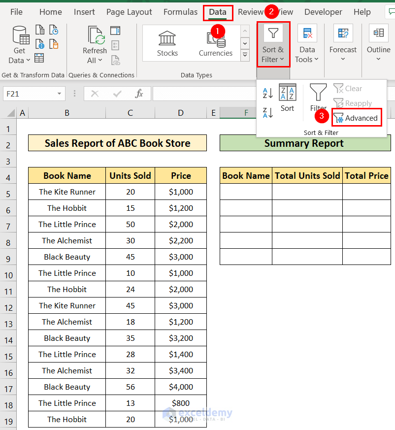
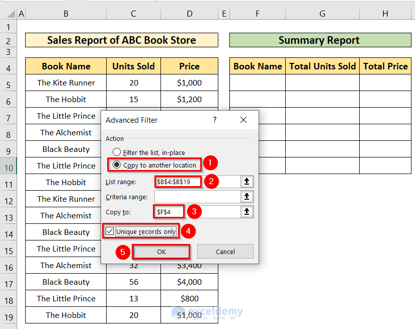
An Advanced Filter window will appear.
➤ Select Copy to another location > we select from cell B4 to B19 as List range.
Select from cells B4 to B19 quickly by clicking on cell B4 and pressing CTRL+SHIFT+Down arrow.
➤ Select cell F4 in the Copy to box > mark on Unique records only > click OK.
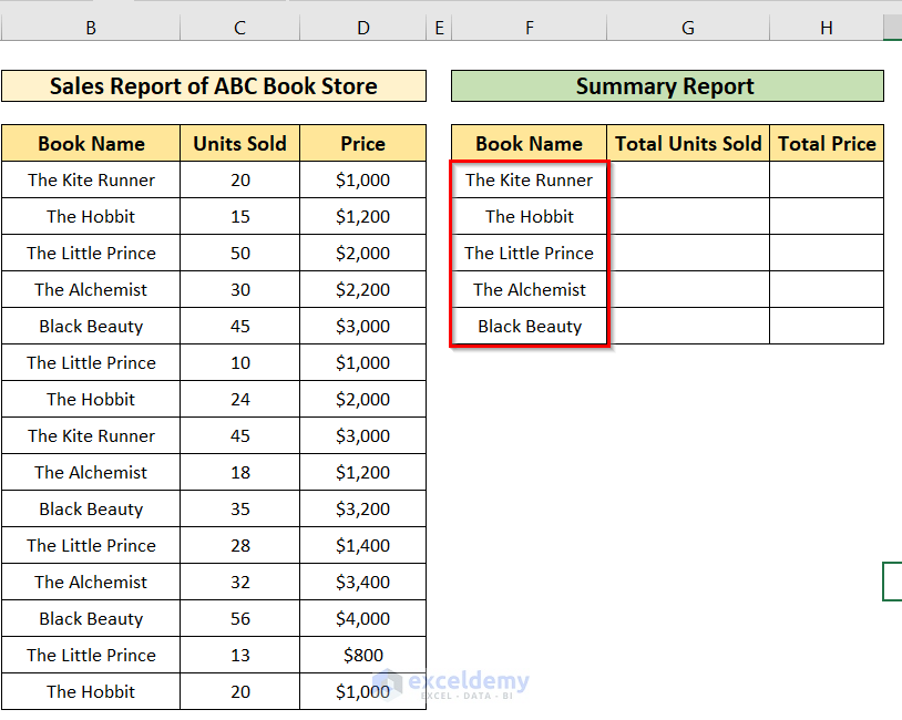
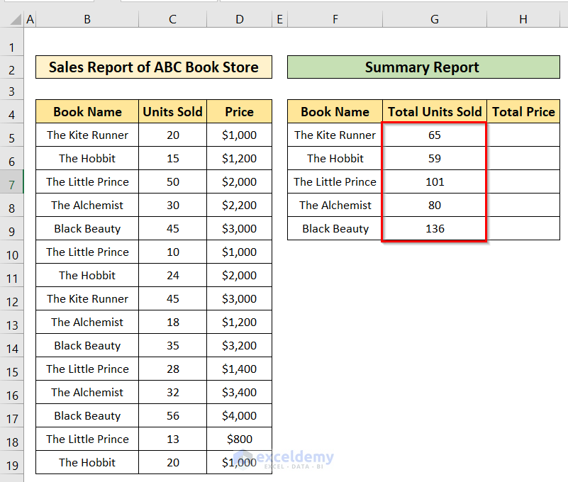
See the unique book name in the Summary Report table’s Book Name column.
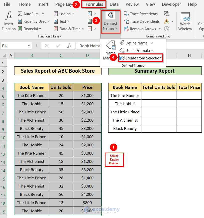
Step 2: Define Names
Define the column names of the Sales Report of ABC Book Store table in the Name Box.
➤ Select the entire dataset of the Sales Report of ABC Book Store table.
Select the entire table quickly by clicking on cell B4 and pressing CTRL+SHIFT+Right arrow+Down arrow.
➤ Go to the Formulas tab > select Defined Names > select Create from Selection.
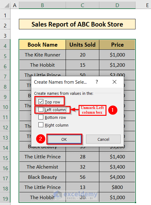
A Create Names from Selection window will appear.
➤ We will unmark the Left column box, and make sure the Top row box is marked > click OK.
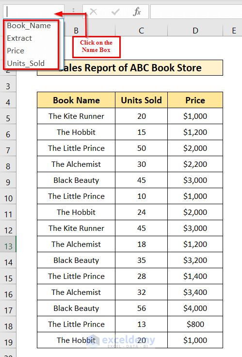
➤ Click on the Name Box, we will see the column names of the Sales Report of ABC Book Store there. We will use these column names in the SUMIF function.
Step 3: SUMIF for Calculation
Calculate the Total Units Sold and Total Price in the Summary Report table. We will use the SUMIF function for this case.
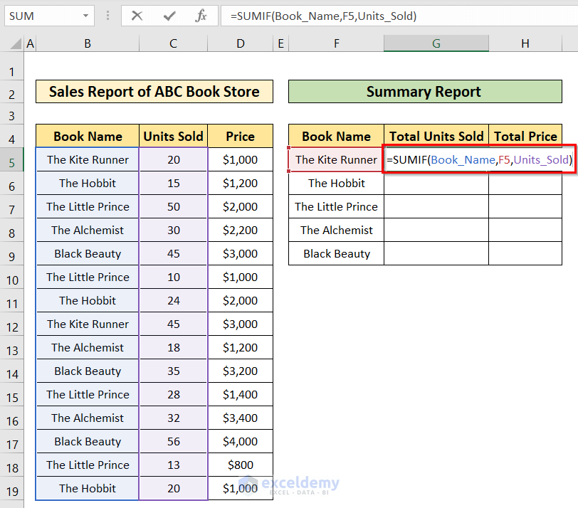
➤ Type the following formula in cell G5.
=SUMIF(Book_Name,F5,Units_Sold)The SUMIF function sums the value in a range that meets specific criteria.
Book_Name is the range of the SUMIF function, F5 is the criterion, and Units_Sold is the sum range.
➤ Press ENTER.
We can see the result in cell G5.
➤ Drag down the formula with the Fill Handle tool.
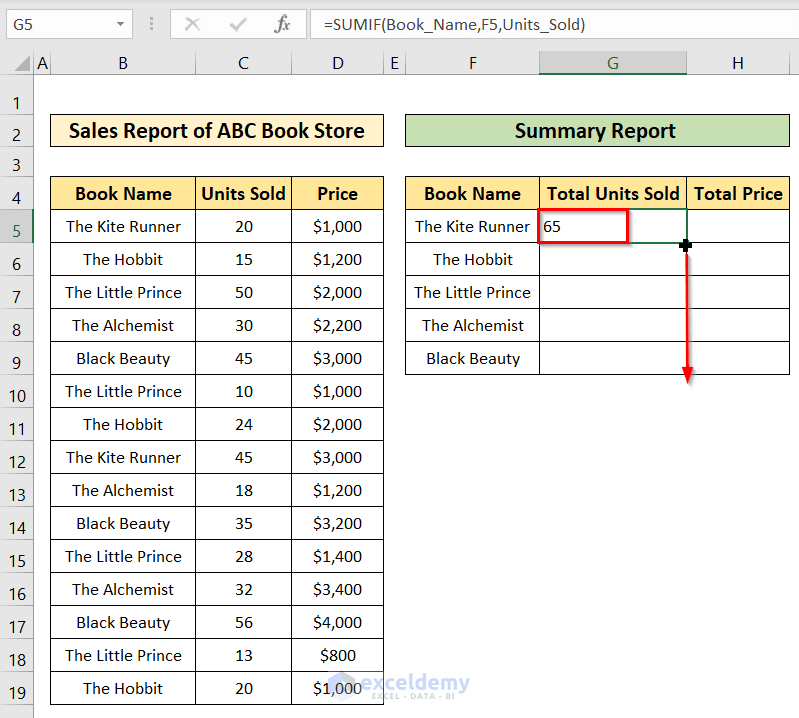
In the Summary Report table, we can see the Total Units Sold for every Book Name.
Calculate the Total Price in the Summary Table.
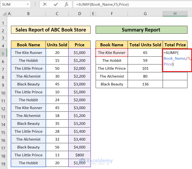
➤ Type the following formula in cell H5.
=SUMIF(Book_Name,F5,Price)Book_Name is the range of the SUMIF function, F5 is the criterion, and Price is the sum range.
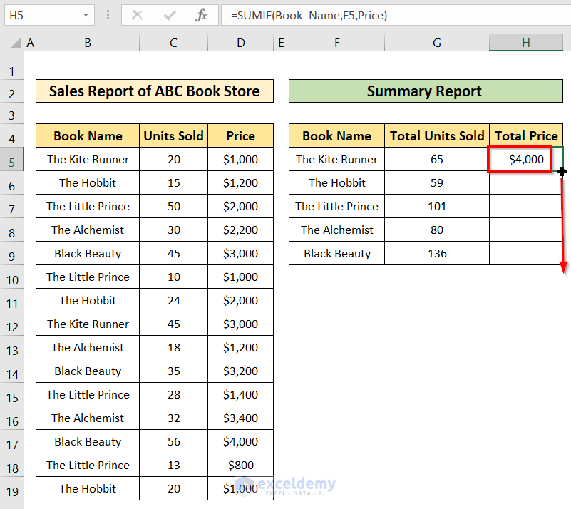
➤ Press ENTER.
See the result in cell H5.
➤ Drag down the formula with the Fill Handle tool.
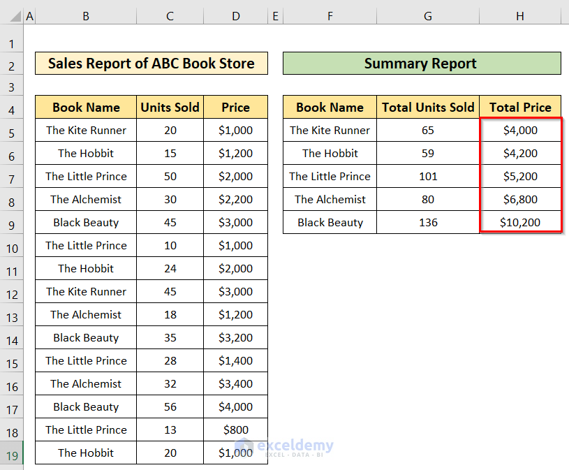
See the Summary Report table with the complete Total Units Sold and Total Price columns.
Step 4: Calculating Grand Total
Calculate the Grand Total of the Summary Report table by using the SUM function.
➤ Type the following formula in cell G10.
=SUM(G5:G9)The SUM function adds up the cells from G5 to G9.
➤ Press ENTER.
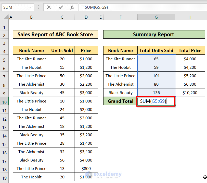
We can see the result in cell G10.
➤ Type the following formula in cell H10.
=SUM(H5:H9)The SUM function adds up the cells from H5 to H9.
➤ Press ENTER.
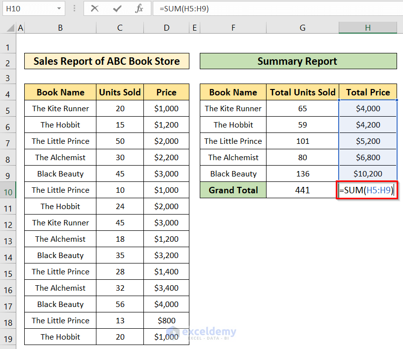
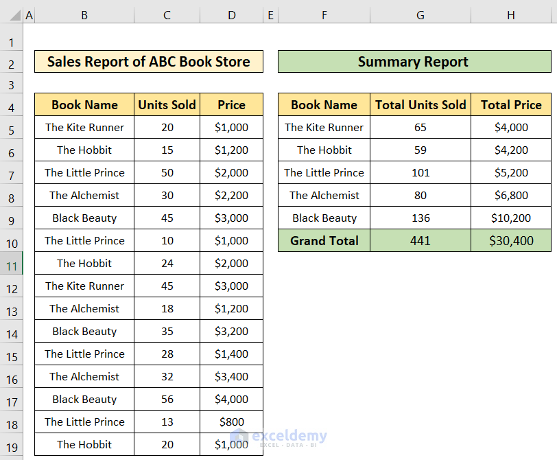
See the complete Summary Report.
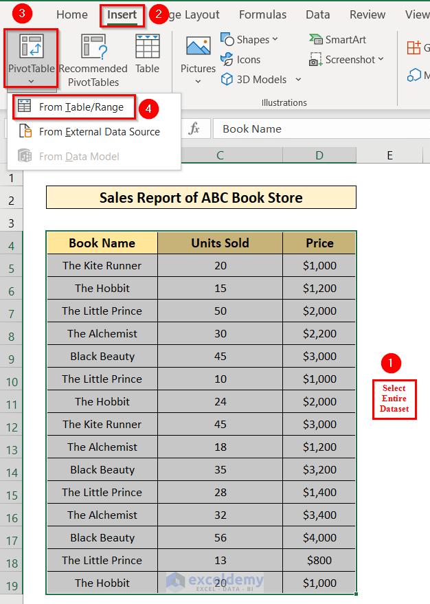
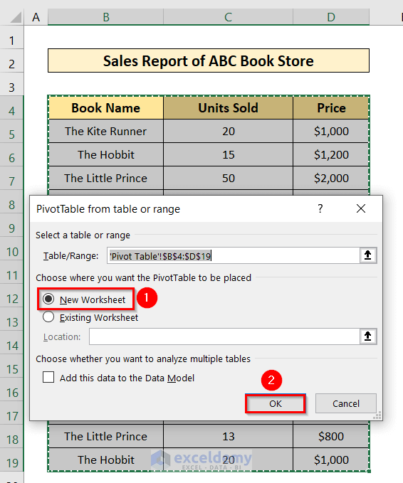
➤ Select the entire dataset of the Sales Report of ABC Book Store table > go to the Insert tab > click on Pivot Table > select From Table/Range.
A PivotTable from table or range window will appear.
➤ Click on Next Worksheet > click OK.
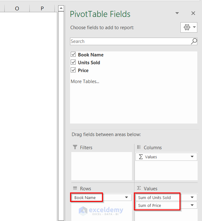
➤ In the PivotTable Fields, we will drag the Book Name in the Rows box and the Units Sold and Price in the Value box.
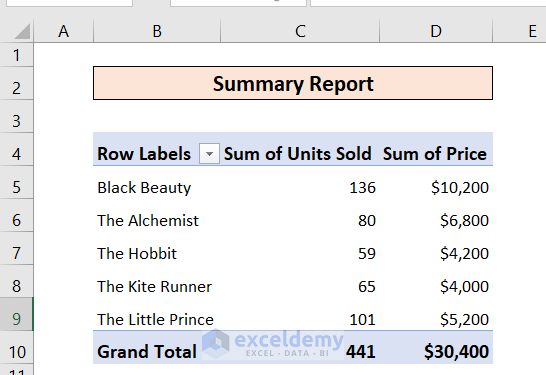
See the Summary Report is created by a Pivot Table.
Download Workbook
Create a Summary Report.xlsx Related Articles How to Make Report Card in Excel How to Automate Excel Reports Using Macros How to Generate Report in Excel using VBA pdf How to Generate Reports in Excel Using Macros Create a Report in Excel as a Table How to Generate PDF Reports from Excel Data How to Generate Reports from Excel Data